PostgreSQL’s EXPLAIN and EXPLAIN ANALYZE commands are the gateway to understanding how a query actually executes. If you’ve ever looked at a query plan and felt like you were staring into the Matrix, this guide will help you make sense of it — using real examples from the Pagila Sample Database.

What EXPLAIN Actually Does

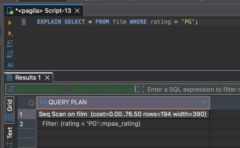
EXPLAIN shows you the query plan the optimizer chooses. It does not run the query — it only predicts how PostgreSQL will execute it.

EXPLAIN SELECT * FROM film WHERE rating = 'PG';

This gives you an estimate of costs, rows, and the path PostgreSQL thinks is best.

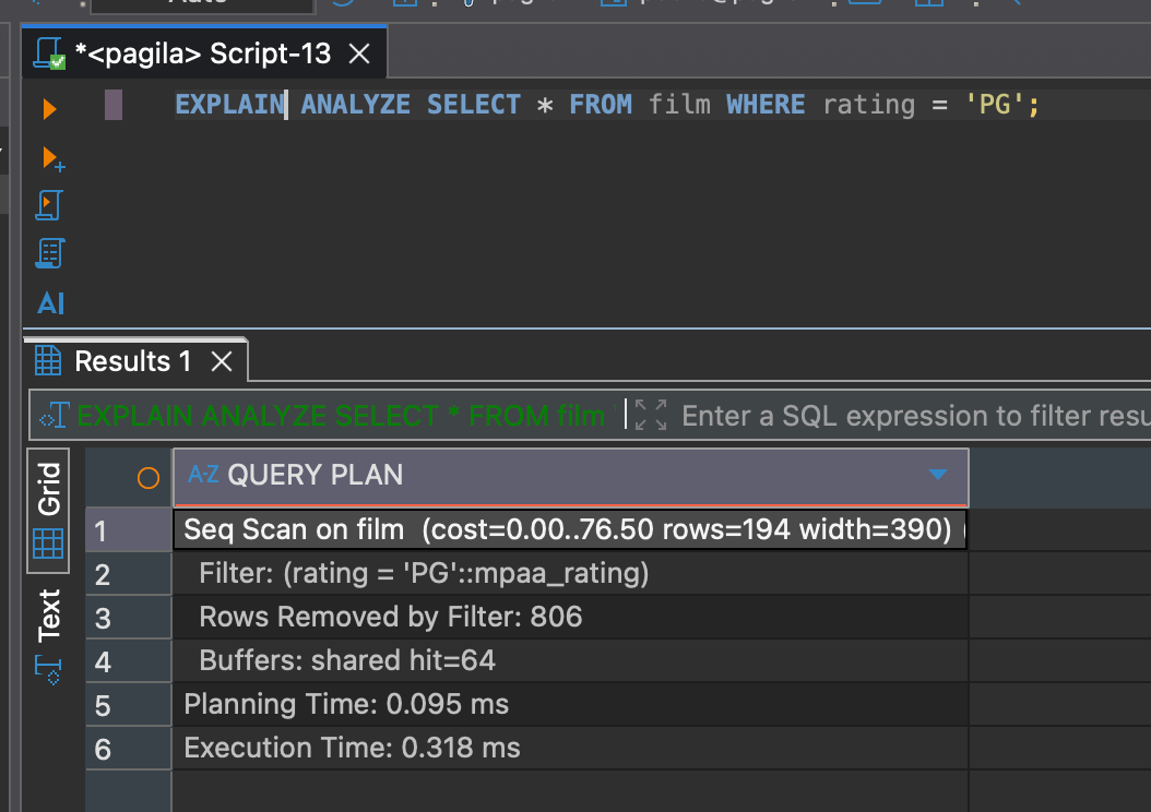
What EXPLAIN ANALYZE Does

EXPLAIN ANALYZE actually runs the query and gives you real execution times and row counts. This is essential for tuning because it shows the truth — not the prediction.

EXPLAIN ANALYZE SELECT * FROM film WHERE rating = 'PG';

This will execute the query and return timing, buffers, and row-level details.

A Simple Pagila Query

Let’s start with a basic lookup in Pagila’s film table:

EXPLAIN
SELECT film_id, title, rating
FROM film
WHERE rating = 'PG';

Let’s break down what this plan is telling us.

Seq Scan on film  (cost=0.00..76.50 rows=194 width=23)
  Filter: (rating = 'PG'::mpaa_rating)

This tells us a few things:

• Seq Scan: PostgreSQL is reading the entire film table.
• cost=0.00..76.50: Estimated cost from start to finish. Higher values usually mean more work.
• rows=194: The planner estimates that 194 rows will match the filter.
• width=23: Estimated size (in bytes) of each output row.
• Filter: The condition applied per row — in this case, rating = 'PG'.

Since there’s no index on rating, PostgreSQL has to scan every row to find matches. This is fine for small tables, but as data grows, this becomes inefficient.

Add an Index and Watch the Plan Change

Let’s create an index on rating to give PostgreSQL a better option.

CREATE INDEX idx_film_rating ON film(rating);

Now run EXPLAIN again:

EXPLAIN
SELECT film_id, title, rating
FROM film
WHERE rating = 'PG';

Result

Bitmap Heap Scan on film  (cost=5.65..72.08 rows=194 width=23)
  Recheck Cond: (rating = 'PG'::mpaa_rating)
  ->  Bitmap Index Scan on idx_film_rating  (cost=0.00..5.61 rows=194 width=0)
        Index Cond: (rating = 'PG'::mpaa_rating)

PostgreSQL switched from a Seq Scan to a Bitmap Heap Scan driven by a Bitmap Index Scan. This still uses the index on rating, but it’s more efficient when the query returns many matching rows. Instead of reading rows one-by-one, PostgreSQL gathers all the matching row locations first, then fetches the table pages in batches. This really starts to shine as the table continues to grow!

This plan tells us:

• Bitmap Index Scan: PostgreSQL uses the index to find all rows where rating = 'PG'.
• Bitmap Heap Scan: PostgreSQL then fetches the matching table pages in efficient batches.
• Recheck Cond: A safety check to ensure the rows still match after being fetched.
• cost=5.65..72.08: New estimated cost — still better than the sequential scan.
• rows=194: The same estimated row count as before.

Reading a Real-World Join Plan

Now let’s step it up and join film with inventory to show available copies.

EXPLAIN ANALYZE
SELECT f.title, COUNT(i.inventory_id) AS copies
FROM film f
JOIN inventory i ON i.film_id = f.film_id
GROUP BY f.title
ORDER BY copies DESC
LIMIT 5;

We should now see something like this:

Limit  (cost=223.91..223.92 rows=5 width=23) (actual time=6.759..6.774 rows=5 loops=1)
  Buffers: shared hit=67 read=30
  ->  Sort  (cost=223.91..226.41 rows=1000 width=23) (actual time=6.744..6.758 rows=5 loops=1)
        Sort Key: (count(i.inventory_id)) DESC
        Sort Method: top-N heapsort  Memory: 25kB
        Buffers: shared hit=67 read=30
        ->  HashAggregate  (cost=197.30..207.30 rows=1000 width=23) (actual time=6.394..6.540 rows=958 loops=1)
              Group Key: f.title
              Batches: 1  Memory Usage: 121kB
              Buffers: shared hit=64 read=30
              ->  Hash Join  (cost=86.50..174.39 rows=4581 width=19) (actual time=2.069..5.216 rows=4581 loops=1)
                    Hash Cond: (i.film_id = f.film_id)
                    Buffers: shared hit=64 read=30
                    ->  Seq Scan on inventory i  (cost=0.00..75.81 rows=4581 width=8) (actual time=1.461..3.611 rows=4581 loops=1)
                          Buffers: shared read=30
                    ->  Hash  (cost=74.00..74.00 rows=1000 width=19) (actual time=0.528..0.529 rows=1000 loops=1)
                          Buckets: 1024  Batches: 1  Memory Usage: 60kB
                          Buffers: shared hit=64
                          ->  Seq Scan on film f  (cost=0.00..74.00 rows=1000 width=19) (actual time=0.024..0.266 rows=1000 loops=1)
                                Buffers: shared hit=64
Planning:
  Buffers: shared hit=185 read=5
Planning Time: 144.378 ms
Execution Time: 8.974 ms

Ok, that looks like a lot! Now how do we read this without going blind?

Here’s the quick interpretation playbook:

• Start at the bottom — query plans always run bottom-up.
• Seq Scan on film and inventory — PostgreSQL is scanning both tables in full to prepare for the join.
• Hash — PostgreSQL builds an in-memory hash table from the film table to speed up the join.
• Hash Join — PostgreSQL joins inventory to film using the hash table (very fast when one side fits in memory).
• HashAggregate — this performs the GROUP BY f.title step, combining rows and counting copies.
• Sort — results are sorted by the computed count in descending order.
• Limit — PostgreSQL returns only the top 5 rows.

When you can identify the bottom scan, the join type, the aggregation step, and the upper sort, the plan suddenly becomes readable instead of overwhelming.

These are the key metrics that actually matter:

• rows vs actual rows — big differences indicate bad estimates or missing statistics.
• actual time — real execution time for each step.
• loops — how many times that node executed.
• Buffers — shows what was read from memory vs disk.
• Hash Cond — the condition used for the hash join.

Conclusion

Learning to read PostgreSQL execution plans comes down to understanding the fundamentals: scans, joins, filters, aggregates, and how estimated rows compare to actual rows. With those pieces in place, both EXPLAIN and EXPLAIN ANALYZE become simple — use EXPLAIN for a quick preview, and EXPLAIN ANALYZE when you need real execution details and performance insight.

The more you practice on the Pagila database and your own workloads, the faster query tuning becomes. Over time, you’ll start to recognize patterns instantly and understand why PostgreSQL chooses certain paths, giving you the confidence to build queries and systems that scale cleanly as your data grows!